Understanding and Measuring Time Delay in an Analytical Instrumentation System
Understanding and Measuring Time Delay in an Analytical Instrumentation System
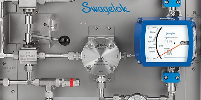
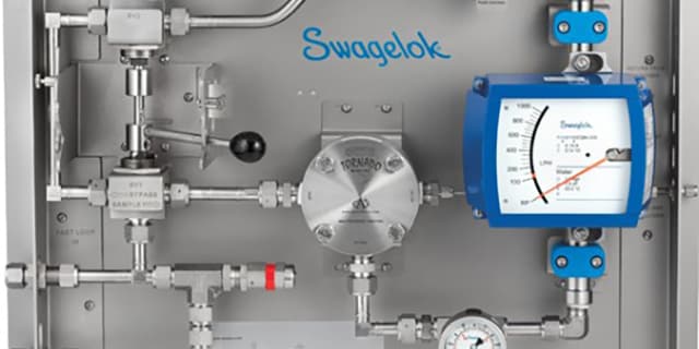
Time delay in sample systems is the most common cause of inappropriate results from process analyzers. Process measurements are instantaneous, but analyzer responses are not. There is always a time delay from the tap to the analyzer. The potential for time delay exists in the following sections of an analytical instrumentation (AI) system, exhibited in the image seen below: process line, tap and probe, field station, transport line, sample conditioning system, stream switching system, and analyzer.

It’s important to understand that time delay is cumulative. It consists of the total amount of time it takes for a fluid to travel from the process line to the analyzer, including time required for final analysis. For example, if the gas chromatograph takes five minutes to analyze a sample, that five minutes must be added not only to the time delay in the sampling conditioning system and stream switching system, but also to the time delay in the transport lines, field station, tap, and probe. This subtotal must be then added to the amount of time it takes for the fluid to travel from the process unit being monitored to the tap. It is the total amount of time from the process unit being monitored through to the analyzer that counts.
Unfortunately, time delay is often underestimated, not accounted for, or misunderstood. In many cases, time delay is invisible to analyzer specialists and technicians, who are focused on making the sample suitable for the analyzer. Analyzer specialists may assume that the analytical measurement is instantaneous. However, sampling systems often fail to achieve the industry standard of a one-minute response, creating ample opportunity for time delay. It’s always best to minimize time delay, even for long cycle times, but delays extending beyond the industry standard are not necessarily a problem. The process engineer must determine acceptable delay times based on process dynamics.
Time delays become an issue when they exceed a system designer’s expectations. A poor estimate or wrong assumption about time delay will result in inferior process control. Understanding the causes of time delay and learning to calculate or approximate a delay within a reasonable margin of error can both reduce delay and improve overall system responsiveness.
Placing Process Lines, Taps, Fast Loops, and Transport Lines for Maximum Effectiveness
To reduce time delay, it is generally best to locate the tap closest to the analyzer, although this is not always feasible. The tap should be located upstream of sources of delay, such as drums, tanks, dead legs, stagnant lines, or redundant or obsolete equipment (which should be eliminated to improve flow). In some cases, location of the tap cannot be specified near the process analyzer due to the previously mentioned variables. If the tap is a long distance from the analyzer, a fast loop is recommended to quickly deliver fluid to the analyzer. If properly designed, flow in the fast loop will be much faster than the flow through the analyzer lines.
Reducing Pressures to Decrease Time Delay
When used with a gas, a field station is a means of reducing pressure in the transport lines or fast loop. Given the same flow rate, the time delay in the transport lines is reduced in direct proportion to the reduction in absolute pressure. At half the pressure, there is half the time delay. The field station should be located as close to the tap as possible. The sooner the pressure is dropped, the better.
With a liquid sample, a regulating field station is not employed. It is better to keep liquids at a high pressure to avoid the formation of bubbles. When a liquid sample is analyzed as a gas, a vaporizing regulator may be used at the field station. However, this will cause considerable time delay. As the fluid changes from liquid to gas, volume will increase dramatically. The rate of increase will depend on the liquid’s molecular weight.
Typically, the measured vapor flow after the regulator will be >300 times the liquid flow before the vaporizing regulator. For example, with a vapor flow of 500 cm3/min, the liquid flow may be less than 2 cm3/min. Therefore, the liquid will take 25 minutes to travel through 10 feet of one-quarter inch tubing. To reduce this time, we must reduce the volume of the tubing preceding the regulator. For example, with only one foot of one-eighth inch tubing, it would take only 30 seconds for the liquid to reach the regulator. To this time, however, we must add time delay in the probe. The narrower the probe, the faster the response.
Another means of attaining a faster response is to place the vaporizing regulator closer to the analyzer location. Install a regulator after the fast loop filter with a second liquid fast loop to ensure that positive flow continues right up to the vaporizing regulator. The objective is to minimize slow-moving liquid volume going to the regulator.
Stream Switching
To avoid as much time-delay as possible, stream switching assemblies must work fast, quickly purging old sample material while moving the new stream to the analyzer. Double-block-and-bleed (DBB) valve configurations, which are available today in conventional components or miniature, modular designs, provide a means of switching streams with minimal deadlegs and no cross-stream contamination from leaking valves.
A traditional DBB configuration is the cascading DBB, seen in the diagram below. The cascading DBB eliminates deadlegs by using a second block valve instead of a tee piece.

When using a DBB cascading configuration, the flow path needs to be taken into consideration as this configuration can lead to pressure drop and slower flow. The pressure drop may be estimated by looking up the product’s Cv, which is a measure of the resistance to flow. The lower the Cv, the greater the pressure drop, resulting in a lower flow rate.
In the DBB cascading configuration, the primary stream – Stream 1– does not cause excessive pressure drop but Stream 2, Stream 3, and so on create increasing amounts of pressure drop and a longer flow path, resulting in progressively longer travel times to the outlet. The result is inconsistent delivery times from the different streams, making it difficult to set consistent purge times for all streams.
The DBB configuration with an integrated flow loop, shown in the diagram below, enables all the advantages of the DBB cascading configuration while ensuring minimal pressure drop consistently across all streams. The Cv for each stream – and therefore the delivery time for each stream – will be the same. Note that a component with a Cv of 0.3 will cause one-third the pressure drop of one with a Cv of 0.1.

Sample Conditioning Systems
The sample conditioning system prepares the sample for analysis by filtering it, ensuring it is in the right phase, and adjusting pressure, flow, and temperature. To do this in a small form factor, the system uses many relatively-small components, including gauges, regulators, variable area flowmeters, flow controllers, check valves, control valves, and ball valves. Frequently, miniature modular components are also used as a compact solution for tight spaces. These top-mounted components are manufactured to ANSI/ISA 76.00.02 standard, according to the New Sampling/Sensor Initiative (NeSSI). As with the stream switching valves, internal volume is not as important as pressure drop. When choosing components, you should compare the Cv provided by the manufacturer.
Other components used in sample conditioning systems, such as filters, knockout pots, and coalescing filters, may cause significant time delay because they allow incoming samples to mix with old samples. Improve time delay by clearing out a filter or knockout pot so that 95 percent of the old sample is gone. Unfortunately, this requires three times the volume of the component. That’s assuming the inlet and outlet are adjacent, as shown in the diagram below.

Consider a filter with an inlet and outlet configured in the diagram. If the flow rate is 100 cm3/min and the filter’s volume is 100 cm3, it will take three minutes to ensure that 95 percent of the old sample has been flushed out. Therefore, to ensure an accurate sample, three minutes must be added to the time delay calculation for this AI system. These same formulas may be applied to mixing volumes in the process line.
Analyzer
Generally, a gas chromatograph will take five to 10 minutes to analyze the sample. Infrared and ultraviolet analyzers work much faster, completing analyses within seconds. An analyzer specialist, technician, or engineer should know the amount of time required for the analyzer to process a sample. That time will be added to the estimates discussed above for the total time delay from tap through the analyzer.
In Conclusion
The total time delay as calculated with the tools described should provide an estimate within a reasonable margin of error. Remember that it is the total time from the process being monitored to the analyzer that matters, and that all components making up this delay must be added to the total. Time delay is an issue that deserves the analyzer specialist’s close scrutiny. Incorrect assumptions about the sample time, particularly for typical trouble spots, such as the probe or a vaporizing regulator in the field station, will undermine all the analyzer specialist’s hard work and render the analyzer ineffective. Analyzer specialists, in collaboration with their fluid system provider or consultant, can improve time delays by making intelligent choices about components and configurations with respect to the location of the tap, fast loop set-up, appropriate tubing diameters, and stream switching configurations.
Related Articles
How to Use a Regulator to Reduce Time Delay in an Analytical Instrumentation System
Time delay is often underestimated or misunderstood in analytical systems. One way to mitigate this delay is with a pressure-controlled regulator. Learn how manage your analytical system’s time delay with tips from the experts at Swagelok.
4 Areas to Inspect When Measuring Time Delay in Sampling Systems
In a process analyzer sampling system, there is always a time delay before you obtain a reading. However, underestimating this time delay can lead to inferior process control. Learn which four areas you should closely inspect to diminish time delays.
Sampling Systems: 8 Common Process Analyzer Accuracy Challenges
Sampling systems expert and veteran industry instructor Tony Waters offers plant managers and design engineers tested ways to identify and resolve 8 common challenges for process analyzer accuracy.